In the era of big data, time series analysis has emerged as a crucial technique for forecasting and understanding temporal data. Time series data refers to a sequence of observations collected at regular intervals over time. These data points are often correlated and can reveal underlying patterns, trends, and seasonality. Analyzing and forecasting time series data have wide applications, from finance and economics to weather forecasting and business planning.
In this blog, we will dive into the world of time series analysis, exploring various techniques and methodologies. We will also provide practical examples with code snippets to demonstrate their implementation. So, let’s embark on our journey to unravel the hidden insights within temporal data!
What is Time Series Analysis?
Time series analysis involves the study of data points ordered by time to identify patterns and make predictions about future values. It plays a vital role in understanding dynamic processes and making informed decisions based on historical trends.
In time series analysis, we often encounter two main components:
Trend: The long-term movement or tendency of the data to increase or decrease over time.
Seasonality: The repeating patterns or variations that occur at regular intervals.
Let’s start with a simple example to gain an understanding of these components.
Example: Analyzing Temperature Trends
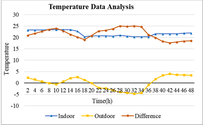
Suppose we have collected temperature data for a specific location over several years. We can start by visualizing the data to observe any trends or seasonality. In this example, we’ll use Python and its libraries to analyze the data.
Python
# Importing libraries
import pandas as pd
import numpy as np
import matplotlib.pyplot as plt
# Generating sample data
np.random.seed(42)
date_rng = pd.date_range(start=’2010-01-01′, end=’2020-12-31′, freq=’D’)
temperature_data = np.random.normal(loc=20, scale=5, size=len(date_rng))
# Creating a DataFrame
temperature_df = pd.DataFrame({‘Date’: date_rng, ‘Temperature’: temperature_data})
# Setting ‘Date’ column as the index
temperature_df.set_index(‘Date’, inplace=True)
# Visualizing the data
plt.figure(figsize=(12, 6))
plt.plot(temperature_df.index, temperature_df[‘Temperature’], label=’Temperature’)
plt.xlabel(‘Date’)
plt.ylabel(‘Temperature (°C)’)
plt.title(‘Temperature Time Series’)
plt.legend()
plt.show()
The code above indicates a few temperature fluctuations over time. The data seems to have an increasing trend indicating that the temperature has risen gradually over the years. It also indicates some periodic ups and downs, suggesting the presence of seasonality. Next, we will look into techniques to extract these components and make predictions.
Decomposition of Time Series
Decomposing a time series involves breaking it down into its constituent parts: trend, seasonality, and residual (random fluctuations). It allows us to analyze each component separately and understand their individual contributions to the overall behaviour of the time series.
Example: Decomposing Temperature Data
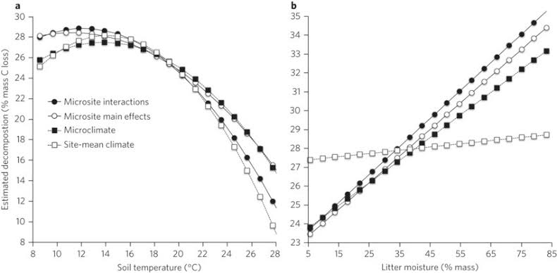
In Python, we can use the seasonal decomposition of time series (STL) method to perform decomposition. The ‘statsmodels’ library provides an implementation for this.
Python
from statsmodels.tsa.seasonal import STL
# Decomposing the time series
stl = STL(temperature_df[‘Temperature’], seasonal=13)
result = stl.fit()
# Plotting the decomposition
plt.figure(figsize=(12, 8))
plt.subplot(4, 1, 1)
plt.plot(result.trend)
plt.title(‘Trend’)
plt.subplot(4, 1, 2)
plt.plot(result.seasonal)
plt.title(‘Seasonal’)
plt.subplot(4, 1, 3)
plt.plot(result.resid)
plt.title(‘Residual’)
plt.subplot(4, 1, 4)
plt.plot(result.trend + result.seasonal + result.resid)
plt.title(‘Reconstructed’)
plt.tight_layout()
plt.show()
This above code is meant to separate components of the temperature time series. By analyzing these components, we can make more accurate predictions and better understand the data’s underlying patterns.
Trend Analysis
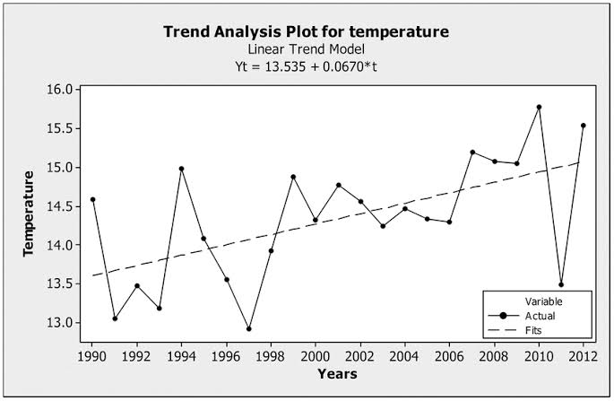
Trends are essential characteristics of time series data, as they help us comprehend the general direction in which the data is moving over time. There are several ways to identify and analyze trends, including:
Moving Averages: This method calculates the average of a fixed number of data points within a sliding window. It smooths out short-term fluctuations and highlights long-term trends.
Exponential Smoothing: This technique assigns exponentially decreasing weights to historical data, emphasizing recent observations more than older ones.
Linear Regression: Using a regression model, we can fit a line to the data points and estimate the slope (trend) and intercept (initial value).
Let’s explore an example of using moving averages to identify trends in our temperature data.
Example: Analyzing Trends with Moving Averages
In this example, we will calculate the moving average of the temperature data to reveal its underlying trend.
Python
# Calculating 30-day moving average
temperature_df[‘Moving_Avg’] = temperature_df[‘Temperature’].rolling(window=30).mean()
# Plotting the original data and moving average
plt.figure(figsize=(12, 6))
plt.plot(temperature_df.index, temperature_df[‘Temperature’], label=’Temperature’)
plt.plot(temperature_df.index, temperature_df[‘Moving_Avg’], label=’Moving Average’, color=’red’)
plt.xlabel(‘Date’)
plt.ylabel(‘Temperature (°C)’)
plt.title(‘Temperature Time Series with Moving Average’)
plt.legend()
plt.show()
This code will result in observations that the moving average smoothens out the fluctuations and highlights the long-term increasing trend more clearly.
Seasonality Analysis
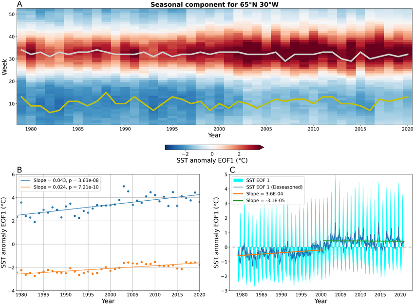
Seasonality refers to repeating patterns that occur at regular intervals in a time series. It could be daily, weekly, monthly, or yearly patterns, depending on the nature of the data. Identifying and understanding seasonality can aid in predicting future values and making informed decisions.
There are various methods to analyze seasonality, including:
- Seasonal Subseries Plot: This plot divides the time series data into individual seasons, allowing us to observe patterns for each season separately.
- Autocorrelation Function (ACF): ACF measures the correlation between observations at different time lags. It can reveal seasonality patterns.
- Seasonal Decomposition: As shown in the previous example, decomposition can help extract the seasonal component from the time series data.
Let’s create a seasonal subseries plot for our temperature data.
Example: Analyzing Seasonality with Seasonal Subseries Plot
In this example, we will create a seasonal subseries plot to visualize the seasonality patterns in the temperature data.
Python
# Creating a seasonal subseries plot
temperature_df[‘Month’] = temperature_df.index.month
temperature_df[‘Day’] = temperature_df.index.day
plt.figure(figsize=(12, 8))
for month in range(1, 13):
plt.subplot(4, 3, month)
plt.plot(temperature_df[temperature_df[‘Month’] == month][‘Day’],
temperature_df[temperature_df[‘Month’] == month][‘Temperature’])
plt.title(f’Month {month}’)
plt.tight_layout()
plt.show()
This brings about observations that the recurring temperature patterns within each month, indicate seasonality in the data.
Time Series Forecasting
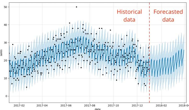
Forecasting is a crucial aspect of time series analysis, as it enables us to predict future values based on historical data. There are various methods for time series forecasting, ranging from simple techniques like moving averages to complex ones like ARIMA (AutoRegressive Integrated Moving Average) and Prophet.
Let’s explore the ARIMA model, one of the most widely used methods for time series forecasting.
Example: Forecasting Temperature Data with ARIMA
ARIMA is a combination of three components: AutoRegression (AR), Integration (I), and Moving Average (MA). It captures the dependencies between observations at different time lags and models the seasonality and trend.
Python
from statsmodels.tsa.arima.model import ARIMA
# Fitting the ARIMA model
model = ARIMA(temperature_df[‘Temperature’], order=(2,1,2))
model_fit = model.fit()
# Forecasting future values
forecast_steps = 365
forecast, stderr, conf_int = model_fit.forecast(steps=forecast_steps)
# Creating future date range for the forecast
future_date_rng = pd.date_range(start=’2021-01-01′, periods=forecast_steps, freq=’D’)
# Plotting the original data and forecast
plt.figure(figsize=(12, 6))
plt.plot(temperature_df.index, temperature_df[‘Temperature’], label=’Temperature’)
plt.plot(future_date_rng, forecast, label=’Forecast’, color=’red’)
plt.fill_between(future_date_rng, conf_int[:, 0], conf_int[:, 1], color=’pink’, alpha=0.3)
plt.xlabel(‘Date’)
plt.ylabel(‘Temperature (°C)’)
plt.title(‘Temperature Forecast with ARIMA’)
plt.legend()
plt.show()
This will go on to indicate that ARIMA has captured the overall trend and seasonality, providing valuable insights into the temperature’s future behaviour.
Conclusion
Time series analysis is a powerful tool for understanding, forecasting, and making decisions based on temporal data. We explored various concepts, from decomposing time series into trend, seasonality, and residual components to forecasting using the ARIMA model.
Remember that time series analysis requires careful consideration of data stationarity, model selection, and parameter tuning. Additionally, there are advanced techniques like Prophet, LSTM (Long Short-Term Memory), and seasonal decomposition with multiple seasonality (STL-M) that can be explored for specific use cases.




Add comment