Introduction
Based on NumPy, Pandas is one of the most popular and robust data analysis libraries in Python. Data analysts, data scientists, and machine learning engineers utilize it essentially every day for projects involving data wrangling, data manipulation and data visualization. In this tutorial, we’ll be using an actual dataset to perform data analysis so you can get started with Pandas and utilize it in your own projects.
Getting started
Installation
Pandas must be installed first before you can use it in your system:
| pip install pandas conda install pandas |
Once installed, it is now ready to be imported in the kernel or notebook:
| import pandas as pd |
Importing libraries
It is useful to import a few required libraries before working with Pandas, such as NumPy for data processing, and matplotlib and seaborn for data visualization.
To perform mathematical array operations:
| import numpy as np |
To create interactive, fully-functional visualizations:
| import matplotlib.pyplot as plt import seaborn as sns |
Working with Data
Pandas offers primarily two types of data structures: series and dataframes. These are designed in a way to make data fast and easier to analyze.
Series
Pandas series is a one dimensional array object of key-value pairs of integers, strings, floats, and other data types. Each element (value) of a series is assigned a unique label, often known as an index or key. Series are often used in data manipulation tasks.
To create a series in pandas, we use pandas.Series():
| import pandas as pd # initialize the series object num = pd.Series([12, 3, 2, 8]) print(num) |
| 0 12 1 3 2 2 3 8 dtype: int64 |
DataFrame
However, dataframes have a two-dimensional structure that is similar to a spreadsheet or table with rows and columns. A dataframes is basically an arrangement of two or more series, with distinct data types, such as name (string), age (int), and date_of_birth (datetime), in each column.
To create a dataframe in pandas, we use pandas.DataFrame():
| import pandas as pd customers = {‘name’: [‘Zeke’, ‘Alex’, ‘Keith’, ‘Elen’], ‘age’: [65, 40, 30, 28], ‘year’: [1958, 1983, 1993, 1995]} df = pd.DataFrame(customers) |
| age name year 0 65 Zeke 1958 1 40 Alex 1983 2 30 Keith 1993 3 28 Elen 1995 |
Loading and Saving Data
Pandas allows us to import and store data in different formats such as CSV and Excel files and connect to databases like SQLite as well.
| # load the data df = pd.read_csv(‘file.csv’) df = pd.read_excel(‘file.xlsx’, sheet_name=‘data’) # save the data df.to_csv(‘output.csv’) df.to_excel(‘output.xlsx’) |
Using SQLite:
| # connect to databases import sqlite3 conn = sqlite3.connect(‘data.db’) query = “SELECT * FROM table_name” df = pd.read_sql_query(query, conn) # save the databases df.to_sql(‘data’, conn, if_exists=‘replace’, index=False) df.to_sql(‘data’, conn, if_exists=‘replace’, index=False) # close the connection conn.close() |
Data Analysis with Pandas
Now that we understand the fundamentals, let’s proceed to utilize pandas for exploratory data analysis (EDA) processes. EDA involves several data analysis techniques, such as :
- Data collection: This includes collecting a significant amount of data from various sources like csv, xlsx files, SQL databases or APIs for analysis.
- Data exploration: It provides a brief overview of the dataset to comprehend its size, distribution, datatype of variables and key metrics.
- Data cleaning: Identifying and handling missing and duplicate data, eliminating irrelevant columns, and making the data consistent for better results.
- Data manipulation: Applying techniques like normalization and standardization to transform data in accordance with the requirements of our project. This is a typical approach for machine learning projects, you can learn more about it here.
Data Exploration
We are going to use this dataset from Kaggle. The CSV file can be downloaded and used locally in your Jupyter notebook, or it can be used directly via Kaggle notebooks, choose the one you prefer and load the dataset:
| import pandas as pd import numpy as np import matplotlib.pyplot as plt import seaborn as sns df = pd.read_csv(‘data.csv’) |
.head() allows us to peek into the first 5 rows of the dataset:
| df.head() |

.shape() returns a tuple of two elements, total number of rows and columns, respectively. This helps to understand the dataset size:
| df.shape() |
| >> (4340, 8) |
There are 4340 rows and 8 columns in the dataset.
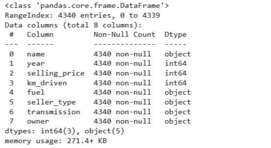
The .info() and .describe() method provide a summary of numerical data and helps with data types and distribution of data, respectively:
| df.info() |
| df.describe() |
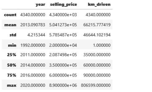
By default, the .describe() method only returns numerical variables. To look for ‘object’ columns:
| df.describe(include=‘object’) |

To check for missing values, we use .isnull() method:
| # sum of missing values in each column
df.isnull().sum() |
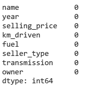
This dataset has no null values. Awesome!
To check for duplicate data, we use .duplicated():
| # sum of duplicate rows df.duplicated().sum() |
| >> 763 |
There are 763 duplicate rows in this dataset.
In the following section we will learn how to deal with duplicates and missing data in our dataset, as these values can significantly affect our analysis.
Data Cleaning
Handling missing data
Too much missing data in the dataset can influence the findings of our analysis. In order to address such circumstances, mean or median value of the respective column can be used to fill in the missing data points.
The choice of whether the mean or median value should be chosen depends on the data to be processed. Suppose that our data is highly skewed, the mean value is not a reliable indicator of central tendency in this case. Therefore we will use the median value to fill the missing data.
| median_col = df[‘col’].median() # filling missing values df[‘col’].fillna(median_col, inplace=True) |
Handling duplicate data
For duplicate rows, we can simply use the drop_duplicates() method, which eliminates all the repetitive rows except the first occurrence:
| df_clean = df.drop_duplicates() df_clean.shape |
| >>(3577, 8) |
| # to modify the original dataframe, set inplace to ‘True’ df.drop_duplicates(inplace=True) |
In this step, a good practice is to create a copy of the dataset to protect the original dataset from any unintended data losses.
Removing irrelevant columns
When performing data analysis, columns like customer reviews or product descriptions are not necessary. We can drop such columns to keep the data clean and easier to explore.
| df = df.drop([‘customer_reviews’], axis=1) |
Data Manipulation
Data manipulation and transformation include tasks that prepare our data for analysis, such as aggregating, filtering and sorting data, as well as creating new columns from pre-existing ones.
Aggregate functions
| # total selling price: total_selling_price = df[‘selling_price’].sum() # average distance covered: average_km_driven = df[‘km_driven’].mean() # number of cars for each fuel type: fuel_counts = df[‘fuel’].value_counts() |
Sorting a DataFrame
Sorting is useful when we are trying to understand trends and patterns among different variables:
| df.sort_values(by=‘selling_price’, ascending=True, inplace=True) |
Filtering a DataFrame
| year_below_2000 = df[df[‘year’] < 2000] len(year_below_2000) >> 29 |
29 data values are available for vehicles registered before the year 2000.
Grouping a DataFrame
| by_price = df.groupby(‘fuel’)[‘selling_price’].mean().reset_index() by_price |
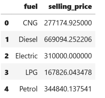
On average, diesel cars have a higher selling price compared to petrol cars, considering the factors like market demand and efficiency of fuel.
Data Visualization
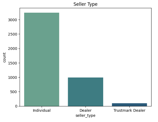
Data visualization libraries like Matplotlib, Seaborn and Plotly offer various plots, graphs and visuals that can be employed with pandas.
Here are a few examples:
| sns.countplot(data=df,x=“seller_type”,palette=“crest”) plt.title(“Seller Type”) plt.show() |
| sns.lineplot(data=df,x=‘year’,y=‘selling_price’,hue=‘fuel’) |
Predictive Analytics
In machine learning, data analysis takes a step further to carry out feature engineering using different techniques like:
- Standardization and normalization to keep variables on the same scale.
- Principal Component Analysis (PCA) to reduce data complexity by dimensionality reduction in huge datasets.
- NLP methods like TF-IDF and bag of words to transform textual data into numerical data.
- Time series analysis for forecasting datetime variables, and more.
Conclusion
This tutorial comes to an end after going over the main concepts behind data analysis processes. Pandas offers a comprehensive documentation that you can explore and try doing projects on your own. All you need is to get some data from Kaggle, GitHub or any online dataset providers and you are ready to go.






Add comment