Linear Regression Analysis: A Beginner's Guide

Jump to

Introduction

Linear regression is a supervised machine learning technique where the target (dependent variable) forms a linear relationship with the features (independent variables). This analysis helps one to predict the value of the target based on the feature sets.

For example, in market analysis, linear regression can be used to predict future sales and discover effective marketing strategies, to predict the probability of a weather forecast, to estimate stock values, and so on.

As a data scientist, learning linear regression can help you understand the relationship between different variables and hence select the most effective ones.

It also aids in providing detailed insights about the dependent and independent variables.

Basics of Linear Regression

Regression analysis assists us in establishing models using target and feature variables. It is used where the target or dependent variable is numerical or continuous data.

Regression analysis is majorly divided into two types, linear regression and logistic regression. In this blog, we will learn about linear regression.

In linear regression, the goal is to simply minimize the sum of mean-squared error for each data point. To put it mathematically,

y = mx + c

where y -> dependent variable (target)

m -> slope of the equation (coefficient)

x -> independent variable (feature)

c -> intercept

In this case, linear regression, a statistical technique will help us to find a better fit for our coefficient values. These numbers are then used to predict our target variable.

Components of Linear Regression

Dependent and independent variables

Dependent Variable (y): It is the value that needs to be determined using the independent variables. In regression analysis, it is also known as the target variable or the outcome.

Independent Variables (X): These are the variables from the dataset that are used to calculate y. It is also referred to as feature variables.

When a regression analysis uses a single independent variable, it is said to be a simple linear regression. A multiple linear regression analysis, on the other hand, is formed when more than one variable is used to predict the dependent variable.

Regression coefficients and the intercept

Regression coefficient: The regression coefficient or slope coefficient is essentially the value that measures the extent or strength of the relationship between the target and feature variables X and y. It determines the slope of our regression line.

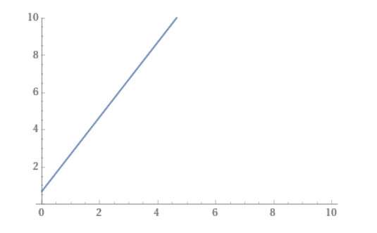
Consider the following regression line equation:

y = 0.7 + 2X

Here the regression coefficient is +2.

The positive and negative signs will determine the nature of the relationship between the input variable (X) and the output variable (y).

If the regression coefficient is positive, y increases as X increases.

If the regression coefficient is negative, y decreases as X increases.

Intercept: In the equation above, the intercept is 0.7. An intercept is the height of the regression line when x = 0.

The y-intercept is the value on the y-axis when x is equal to 0.

Linear Regression Analysis: A Beginner's Guide 1

Assumptions in Linear Regression Model

To obtain consistent and accurate results, the linear regression model makes certain assumptions depending on the dataset. The key assumptions are as follows:

The independent variable (X) and dependent variable (y) exist in a linear relationship.
There should be no little or no correlation between the independent or predictor variables, or it can lead to multicollinearity which makes it difficult to measure the individual impact of these predictors.
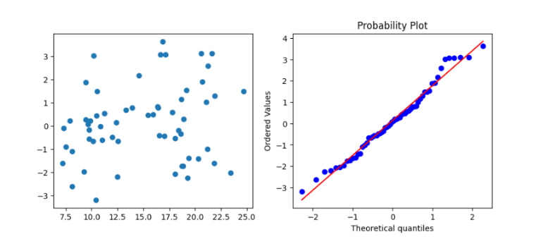
The error terms or residues must follow a normal distribution. One can check for normality by plotting a plot for residues. The absence of normality can also lead to inaccuracy in p-values.
The error terms or residues should not be correlated and should be independent of one another.
The error terms or residues should have constant variance parameters. This ensures that the residues are distributed uniformly across the predicted values.

Data Preprocessing

We must first prepare the data for linear regression analysis before we can begin creating our model. This is known as data preprocessing, which involves data cleaning, data transformation, and normalization. It ensures the accuracy of the model.

The following are some key steps involved in data preprocessing:

1. Check for missing values

Using describe() or info() functions of Python’s pandas’ library, we can get a summary of numerical variables. This can help us count the non-null values.

df.describe()
df.info()

The isnull() function can be used to explicitly check for null values:

df.isnull().sum()

Dropping the column may be a viable choice if the number of missing values is in huge fractions, such as greater than 50%:

df.drop

(col, axis = 1, inplace = True)

2. Check for data types

Incorrect data types, such as ‘object’ for datetime values and ‘string’ for numeric values can cause inconsistency in results. We can check for data types of our variables using .dtypes:

df.dtypes

To convert numeric variables:

df[‘col’] = df[‘col’].astype(float)

To correct datetime variables:

df[‘col’] = pd.to_datetime(df[‘col’])

Building a Linear Regression Model

1. Splitting the data

Once the data is preprocessed, we prepare the dataset for model training. The dataset is separated into training and testing datasets.

Training data: Used as the input set for model building.

Testing data: Used to assess and evaluate the trained model.

For this tutorial, we will be using this company sales dataset from Kaggle.

# import libraries

import numpy as np

import pandas as pd

import matplotlib.pyplot as plt

# Load the dataset
df = pd.read_csv(‘sales_data.csv’)
df.head()

Linear Regression Analysis: A Beginner's Guide 2

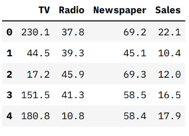
In this dataset df, we will choose ‘Sales’ as the target variable and ‘TV’, ‘Radio’, and ‘Newspaper’ as the feature variables. We will then build a linear regression model that will predict ‘Sales’ based on the other three variables’ values.

# Split the dataset
X = df.drop([‘Sales’], axis=1) # features
y = df[‘Sales’] # target

2. Prepare the training and testing sets

Now that we have defined our target and predictor variables, let’s split the data into distinct sets. We will keep 30% of the data in the testing set and remaining 70% in the training set:

from sklearn.model_selection import train_test_split
X_train,X_test,y_train,y_test=train_test_split(X,y,test_size=0.3,random_state=97)

Check the shape of X and y testing and training sets:

print(‘X_train shape: ‘, X_train.shape)
print(‘X_test shape: ‘, X_test.shape)
print(‘y_train shape: ‘, y_train.shape)
print(‘y_test shape: ‘, y_test.shape)

>> X_train shape: (140,3)

>> X_test shape: (60,3)

>> y_train shape: (140,)

>> y_test shape: (60,)

3. Train the Linear Regression Model

We have our training and testing sets, and we will use the training dataset (X_train, y_train) to train the linear regression model. This is performed using the Scikit-learn library.

Sklearn or Scikit-learn is an efficient machine learning library in Python that provides sophisticated tools for regression, classification, and clustering algorithms, as well as modeling.

# import LinearRegression model from sklearn library

from sklearn.linear_model import LinearRegression

# initiate the model
lr = LinearRegression()

# fit the model into training datasets
lr.fit(X_train,y_train)

4. Model Evaluation

Once the linear regression model is ready, we can use the sklearn.metrics module to evaluate the model against our testing dataset (X_test, y_test), predict the ‘Sales’, and hence check the performance of our model.

Let’s compute the MAE (Mean Absolute Error), MSE (Mean Squared Error), RMSE (Root Mean Squared Error) and the coefficient of determination (R² score) using the evaluation metrics. These are loss functions, which we want to minimize, and they represent how well our model fits the data.

pred = lr.predict(X_test)

from sklearn.metrics import mean_squared_error, r2_score
mse = mean_squared_error(y_test, pred)
mae= mean_absolute_error(y_test, pred)
rmse = np.sqrt(MSE)
rsqe = r2_score(y_test, pred)
print(‘Mean Squared Error: ‘, mse)
print(‘Mean Absolute Error: ‘, mae)
print(‘Root Mean Squared Error: ‘, rmse)
print(‘r square: ‘, rsqe)

>> Mean Squared Error: 2.5617073537905655

>> Mean Absolute Error: 1.272133484712927

>> Root Mean Squared Error: 1.6005334591287261

>> r square: 0.9120817050039508

Our R2 value indicates that our linear regression model is able to explain approximately 91.21% of the variability in the target variable.

To help us understand better, we can plot a probability plot of residuals between the predicted and actual values:

import scipy.stats as stats

def res_plot(y_test, pred):
res = y_test – pred
plt.figure(figsize=(10,4))
plt.subplot(1,2,1)

plt.scatter(pred,res)
plt.subplot(1,2,2)
stats.probplot(res,dist=’norm’,plot=plt)
res_plot(y_test, pred)

Linear Regression Analysis: A Beginner's Guide 3

Calculating the intercept and coefficient of the regression line:

intercept = lr.intercept_
coefficients = lr.coef_
print(‘Intercept: ‘, intercept)
print(‘Coefficient of line: ‘, coefficients)

>> Intercept: 4.7818289462319346

>> Coefficient of line: [0.05352604 0.1024281 0.00181339]

pd.DataFrame(lr.coef_, X.columns, columns=[‘Coefficients’])

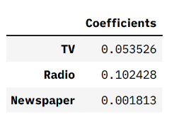
Linear Regression Analysis: A Beginner's Guide 4

The linear regression equation will be:

y = 4.7 + 0.053 * x1 + 0.102 * x2 + 0.001 * x3

5. Plotting the Regression Line

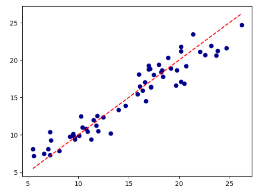
To visualize the regression line, let’s plot a line and scatterplot between our target variable (y_test) and predicted variable (pred) as calculated in our linear regression model above.

The regression line passes through the scatter points in such a way that it minimizes the sum of squared residuals.

plt.scatter(y_test, pred, color=‘darkblue’)
plt.plot([y_test.min(), y_test.max()], [y_test.min(), y_test.max()], ‘r–‘)

Linear Regression Analysis: A Beginner's Guide 5

Overfitting and Underfitting

In Machine Learning, issues like overfitting and underfitting occur that might affect and disrupt the performance of our model.

Overfitting

Overfitting is when a model can’t make accurate predictions due to complexities. This generally happens when the model performs exceptionally well with training data but produces poor outputs with the testing data. To deal with overfitting, we implement methods like model ensemble, cross-validation, and feature selection.

Underfitting

Underfitting is when a model is unable to recognise the trends and patterns in the data because of being overly simple. To deal with underfitting, we can increase model complexity, add more features, and increase the training time of the model.

Conclusion

Linear regression models in regression analysis is a powerful tool for establishing relationships between dependent and independent variables, predictive modeling, and determining the most accurate variables for our target.

We can further expand our knowledge by learning advanced models for high-dimensional and complex datasets.

linear regression regression analysis

Linear Regression Analysis: A Beginner’s Guide

Introduction